Interactive Resources for Schools


This topic takes on average 55 minutes to read.
There are a number of interactive features in this resource:
 Science
The Spearman’s rank correlation coefficient is used when wanting to investigate whether a correlation (positive or negative) exists between two variables. Examples may include comparing the height and weight of individuals, or the rates of smoking and cancer in various countries. Often information of this nature is plotted as a scatter graph, which can help to visualise any potential correlation between two variables:
In the following example, you are investigating the link between the number of hours each day 10 individuals spent revising for a science exam in the week leading up to it, and the percentage score that they attained. Our null hypothesis would state ‘There is no correlation between the number of hours spent revising each day, and the score attained on the exam’.
| Individual | Number of revision hours | Percentage score | Rank A | Rank B |
| 1 | 2.0 | 75 | 5.5 | 6.5 |
| 2 | 1.5 | 72 | 7.0 | 8.0 |
| 3 | 3.0 | 85 | 3.0 | 3.0 |
| 4 | 0.5 | 81 | 10.0 | 4.0 |
| 5 | 2.5 | 75 | 4.0 | 6.5 |
| 6 | 1.0 | 62 | 8.5 | 10.0 |
| 7 | 4.0 | 89 | 1.0 | 2.0 |
| 8 | 3.5 | 78 | 2.0 | 5.0 |
| 9 | 2.0 | 92 | 5.5 | 1.0 |
| 10 | 1.0 | 69 | 8.5 | 9.0 |
The first step is to rank each individual on both the number of hours they spent revising each day (Rank A) and their score (Rank B). When two or more individuals are tied in their score, they are given the average rank for those ranks, for example individuals 1 and 9 were tied at 75%, occupying the 5th and 6th ranks. To ensure we don’t show bias against one of the individuals, we average the ranks, giving them both a rank of 5.5.
Next, we need to find the numerical difference in ranks of each individual by subtracting Rank B from Rank A (represented as d), and then these differences need to be squared (represented as d2).

You may expect more revision would mean a higher score, but is there a statistically significant correlation?
| Individual | Number of revision hours | Percentage score | Rank A | Rank B | d | d2 |
| 1 | 2.0 | 75 | 5.5 | 6.5 | -1.00 | 1.00 |
| 2 | 1.5 | 72 | 7.0 | 8.0 | -1.00 | 1.00 |
| 3 | 3.0 | 85 | 3.0 | 3.0 | 0.00 | 0.00 |
| 4 | 0.5 | 81 | 10.0 | 4.0 | 6.00 | 36.00 |
| 5 | 2.5 | 75 | 4.0 | 6.5 | -2.50 | 6.25 |
| 6 | 1.0 | 62 | 8.5 | 10.0 | -1.50 | 2.25 |
| 7 | 4.0 | 89 | 1.0 | 2.0 | -1.00 | 1.00 |
| 8 | 3.5 | 78 | 2.0 | 5.0 | -3.00 | 9.00 |
| 9 | 2.0 | 92 | 5.5 | 1.0 | 4.50 | 20.25 |
| 10 | 1.0 | 69 | 8.5 | 9.0 | -0.50 | 0.25 |
| Total | 77.00 | |||||
Now we have our value for d2, we can utilise the following formula to calculate the test statistic, rs.

By inputting our data into the equation, we can calculate r:

To determine whether this indicates a statistically significant correlation between our variables, the test statistic must be compared to a table of critical values:
| Critical value | ||
| Sample size | p = 0.05 | p = 0.01 |
| 6 | 0.886 | 1.000 |
| 7 | 0.786 | 0.929 |
| 8 | 0.738 | 0.881 |
| 9 | 0.700 | 0.833 |
| 10 | 0.649 | 0.794 |
| 11 | 0.618 | 0.755 |
| 12 | 0.587 | 0.727 |
| 13 | 0.560 | 0.703 |
| 14 | 0.539 | 0.679 |
The critical value for n = 10 at p = 0.05 is 0.649. As this is larger than our test statistic of 0.533, we can say that there is no statistically significant correlation between the number of hours spent revising each day, and the percentage score on the science exam. Therefore, we accept the null hypothesis.
If we plot the data on a scatter graph:
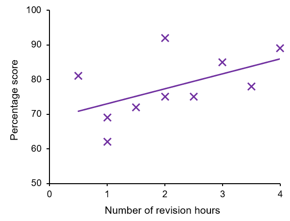
We can see that there does appear to be a positive correlation between the two variables. This highlights why statistical tests are so important, while there appears to be a positive correlation between the two variables, at the statistical significance level of p ≤ 0.05, there is no statistically significant correlation between the variables.