Interactive Resources for Schools


This topic takes on average 55 minutes to read.
There are a number of interactive features in this resource:
 Science
The Student’s t-test utilises the means and standard deviations of two separate samples, comparing them to see if there is a significant difference between the samples. Importantly, there are two different kinds of t-test to utilise depending on the kind of data you have. If both of your samples are from the same individuals, you should use the paired t-test. If your samples are from different individuals, you should use the unpaired t-test
A good way to remember this is to think of how you may construct an experiment to measure the weight of a certain species of bird in spring and in autumn. You could either catch 10 birds in spring, weigh them and then tag them, in the hope that you can catch the same 10 birds in autumn, and weigh them again. As they are the same individuals you are weighing in both seasons, you would use the paired t-test. Alternately, you could catch 10 birds in spring, and catch a different sample of 10 birds in autumn, in which instance you would use the unpaired t-test.

As in the example above, you have caught and weighed 10 individuals from a population of a certain species of bird in spring, and then caught and weighed another 10 individuals from this population in autumn. Remember, with each statistical test we do, we need to keep in mind our null hypothesis, which is this case would be along the lines of ‘the mean weight of the birds will not be different in spring to in autumn’. The weights of the individuals are below.
| Spring | Autumn | ||
| Individual | Weight (g) | Individual | Weight (g) |
| 1 | 20 | 1 | 22 |
| 2 | 18 | 2 | 20 |
| 3 | 15 | 3 | 19 |
| 4 | 19 | 4 | 23 |
| 5 | 20 | 5 | 21 |
| 6 | 20 | 6 | 17 |
| 7 | 21 | 7 | 22 |
| 8 | 20 | 8 | 20 |
| 9 | 16 | 9 | 23 |
| 10 | 15 | 10 | 21 |
| Mean | 18.4 | Mean | 20.8 |
The first thing to do is to calculate the means and standard deviations of both sets of data. In this instance, the means are 18.4g for spring and 20.8g for autumn, while the standard deviations are 2.27g for spring and 1.87g for autumn. For information on calculating standard deviation, see page 3 – Standard deviation.
With the values of mean and standard deviation, we can calculate the t-statistic, which we will use, alongside our known significance level of p ≤ 0.05, to identify whether there is a statistically significant difference between our means.
The t-statistic is calculated through this equation:
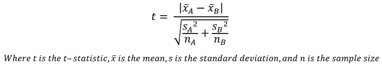
So, by inputting our data points:

Now that we have our t-statistic, we can see whether the difference between the data sets is significant by using a table of critical values. This uses the t-statistic, our significance level (p ≤ 0.05) and the degrees of freedom, which is calculated by taking the sum of both sample sizes (10 for each) and subtracting 2. Hence, we have 18 degrees of freedom. If the t-statistic is greater than the critical value, then we can reject our null hypothesis.
Table of critical values:
| Degrees of freedom | Critical value | |
| p = 0.05 | p = 0.01 | |
| 8 | 2.31 | 3.36 |
| 9 | 2.26 | 3.25 |
| 10 | 2.23 | 3.17 |
| 11 | 2.20 | 3.11 |
| 12 | 2.18 | 3.05 |
| 13 | 2.16 | 3.01 |
| 14 | 2.14 | 2.98 |
| 15 | 2.13 | 2.95 |
| 16 | 2.12 | 2.92 |
| 17 | 2.11 | 2.90 |
| 18 | 2.10 | 2.88 |
| 19 | 2.09 | 2.86 |
| 20 | 2.09 | 2.84 |
Note: When we perform calculations, we often round the result to a sensible number of significant figures (e.g. 2.58 rather than 2.5805258…). However, if we use the number in further calculations, it is best to use as many decimal points as we can (or even the original fraction), to ensure greater accuracy.
Reading off our table of critical values, we can see that the critical value for 18 degrees of freedom at p = 0.05 is 2.10. As this is less than our test statistic of 2.58, we can reject the null hypothesis, and say that there is a statistically significant difference between the weights of this species of bird in spring and in autumn.
In a similar situation, you have caught 10 birds in spring, and then tagged them so you can weigh the same individuals again come autumn. The resulting data would need to be analysed through a paired t-test, as we are comparing data from the same individuals. While conceptually similar, the equation to come to our t-statistic for a paired t-test is quite different to an unpaired t-test.
| Individual | Spring Weight (g) | Autumn Weight (g) | Difference (g)(autumn - spring) |
| 1 | 20 | 20 | 0 |
| 2 | 18 | 21 | 3 |
| 3 | 15 | 18 | 3 |
| 4 | 19 | 19 | 0 |
| 5 | 20 | 21 | 1 |
| 6 | 20 | 19 | -1 |
| 7 | 21 | 23 | 2 |
| 8 | 20 | 20 | 0 |
| 9 | 16 | 18 | 2 |
| 10 | 15 | 17 | 2 |
| Mean | 1.2 | ||
To calculate the t-statistic in paired t-tests, we need to know the mean difference between the two weights, as well as the standard deviation of the difference, which is 1.40. The t-statistic is then calculated using this equation.
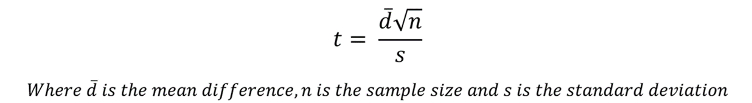
We can input our data, such that:

The number of degrees of freedom for a paired t-test is sample size subtracted by 1, so in this case it is 9. By comparing our t-statistic to our critical table of values seen earlier, we can see it is bigger than the critical value of 2.26 for 9 degrees of freedom at p = 0.05. Thus, we can reject the null hypothesis, and say that there is a statistically significant difference between the weights of these birds between spring and autumn.